
What is the Project?
Polynomial Regression is a technique that provides a way to visualise the relationship between a non-linear dependent variable and one or more independent variables. The project uses a tiny dataset of 20 data points, showing an example of the model and how to create it without using Python libraries. It is a special variant of multi-linear regression that uses a unique characteristic called polynomial features to expand its functionality.
This type of regression is commonly implemented when a dataset follows a curvature that isn't linearly separable.
Components of the Algorithm
We can calculate the Polynomial Regression using equation 2.1. The equation is similar to the one that creates a Multi-Linear Regression. Instead, we multiply each independent variable (\(x\)) by the \(n^{th}\) power, where \(n\) is the degree of the polynomial. Furthermore, \(w\) represents the polynomial coefficients (weights), and \(\epsilon\) is the error rate.
\(\begin{equation} y_i = w_0 + w_1 x + w_2 x^2 + \cdots + w_n x^n + \epsilon \end{equation}\)
(2.1)
Within the algorithm, we use feature engineering to create new input features based on existing ones specified by the degree parameter. The approach is known as polynomial feature expansion and prevents the requirement to edit the original dataset by creating a new one specific to the polynomial regression. For example, using a degree of 3, we create two new variables for each input feature. One is the base value squared, and the second is the base value cubed (table 2.1).
| Coefficient | Base Value | New Value 1 | New Value 2 |
| 1 | 2 | 4 (\(2^2\)) | 8 (\(2^3\)) |
| 1 | 3 | 9 (\(3^2\)) | 27 (\(3^3\)) |
| 1 | 4 | 16 (\(4^2\)) | 64 (\(4^3\)) |
Table 2.1. An example of the values created when using polynomial feature expansion with a degree of 3.
When training the model, we use the Ordinary Least Squares (OLS) method to minimize the sum of squared differences between the independent variables and the predicted dependent variables (equation 2.2).
\(\begin{equation} W = (X^TX)^{-1} X^T y \end{equation}\)
(2.2)
Equation 2.2 updates the polynomial coefficients, where \(X\) is a matrix containing the polynomial feature expansion dataset, and \(X^T\) is the transpose of the matrix. The equation has two components, the inverse of a normal matrix \((X^TX)^{-1}\), and a moment matrix \(X^Ty\), which is a unique symmetric square matrix containing monomials (polynomial values). The moment matrix is calculated using the transpose of the input values multiplied by the dependent variables.
Analysis
To test the algorithm, we used six different degree values: 0, 1, 2, 3, 6, and 10. See figure 3.1 for the results.
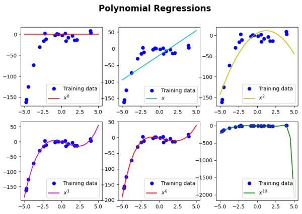
Figure 3.1. Plots of the Polynomial Regression algorithm with six varying degrees: 0, 1, 2, 3, 6, and 10.
As the degree increases from 0 to 6, we gain a better fit for our model. Some of the models massively underfit the data (degrees 0 and 1), while others massively overfit the data (degree of 10). Notice how a degree of 1 performs a standard linear regression because no polynomial features have been created. A degree of 2 provides some underfitting but starts to show a relationship between the data. Lastly, degrees 3 and 6 are an excellent fit for our model, but how do we know which degree is better?
Fortunately, we can evaluate the polynomial regression using a loss function. Loss functions measure the accuracy between the predicted values and actual values. Using these loss functions, we can visualise the difference between the training dataset and the test dataset to identify how the models are performing and find the best degrees for our dataset.
There are many loss functions available, and each one has a different purpose. For example, Mean Absolute Error (MAE) and Mean Squared Error (MSE) provide scores that range from 0 to infinity, which determines the model's effectiveness at prediction values. The lower the score, the better the model. MAE puts all input values on the same scale and can be heavily affected by outliers. Comparatively, MSE penalises outliers, helping the model ignore them when making predictions.
We use the Root Mean Squared Error (RMSE) in this project, the square root of the MSE. RMSE, formulated in equation 3.1, gives a higher weightage to large values when compared to MSE, helping to minimize the total loss value.
\(\begin{equation} RMSE = \sqrt{\frac{1}{N} \sum\limits^{N}_{i=1}(y_i - \hat{y}_i)^2} \end{equation}\)
(3.1)
Equation 3.1 contains a residual (error) which is the subtraction of the actual values (\(y_i\)) by the predicted values (\(\hat{y}_i\)) squared. These are summed together (\(\sum\limits^{N}_{i=1}\)) and then divided by the total number of data points (\(\frac{1}{N}\)).
We can plot the RMSE values for the training loss and validation loss using validation curves (figure 3.2). These loss metrics help determine if our model is overfitting, underfitting or robust. The three cases are defined in more detail below:
- Overfit model - training loss and validation loss divide after a turning point.
- Underfit model - training loss and validation loss don't reach a turning point.
- Robust model - training loss \(\approx\) validation loss, converging to a turning point.
When a model is overfitting, it performs well on the training dataset but not on the test set. Overfit models learn too much of the noise in the data and fit it too well, resulting in a low bias and high variance. Models that have various redundant features are more likely to overfit.
Underfitting is the opposite. Underfit models cannot capture any suitable patterns within the training data, leading to inaccurate predictions with a high bias and low variance. Models that are too simple (have limited features) or learn from a small amount of training data are more likely to underfit.
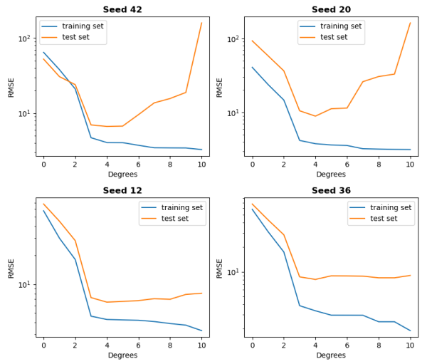
Figure 3.2. Validation curves of four random examples (specified by different seed numbers) of Polynomial Regression training and evaluation using the RMSE.
Within figure 3.2, we train the model on the degree values from 0 to 10 four times. Each graph is slightly different, but all of them provide the same outcome. The degree of 3 provides the most robust model, while two or less represents underfitting and four or higher overfitting.