What is the Project?
Cluster analysis is a form of exploratory data analysis used to find patterns within data by splitting them into clusters. The clusters form homogeneous groups of data based on a given distance function.
K-Means Clustering is one method used in cluster analysis, which takes unlabelled data and combines data points into distinct groups. Being one of the simplest clustering algorithms, it provides a great opportunity for understanding the theory and practice of clustering algorithms.
Throughout this project, we create the K-Means clustering algorithm without the help of any Python libraries, using a dataset of 300 data points representing different dog breeds. The project aims to divide the small dataset into its respective dog breeds based on four distinct traits: height, tail length, leg length, and nose circumference.
Components of the Algorithm
Before creating the K-Means Clustering algorithm, we first need to understand its process and one core component, the centroid. Centroids are unique data points representing the centre of a given cluster. When considered a metric, they reflect the mean value of all the data points around it, specific to its group. They are at the heart of the algorithm and are essential to its implementation, as seen in the following process:
- Specify \(k\) clusters
- Select a random number of centroids \(c\) from the dataset
- Calculate the distance between the centroids and all other data points
- Assign each data point to the closest centroid
- Compute the average of each cluster and set it as a new centroid
- Repeat steps 2 to 5 until the centroids are static
Some of the steps within the algorithm are straightforward and do not need further explanation. As such, we will only discuss two required factors of the algorithm: distance and objective functions.
Distance Functions
Distance functions measure the difference between two points, in our case, data points (\(x\)) and centroids (\(c\)). There are many distance functions available, such as Euclidean, Manhattan, Person Correlation and Spearman Correlation. Due to the simplicity of the K-Means algorithm, we use the Euclidean distance between two vectors, the dataset and the centroids (equation 2.1).
\(\begin{equation} d(x, c) = \sqrt{(x_x - c_x)^2 + (x_y - c_y)^2} \end{equation}\)
(2.1)
The formula compares the distance between a data point (\(x\)) and a centroid (\(c\)) via their \(x\) and \(y\) coordinates. These differences are then squared, summed together, and lastly, we square root the result. The metric provides a method for assigning our clusters using the minimum distances between each centroid and all data points in the dataset.
Objective Functions
Objective functions are types of loss/cost function used to maximize or minimize a numerical value. In clustering algorithms, we want to reduce the variance (sum of squared distances) between each cluster of data. The smaller the variation, the higher the similarities between the data points in their group. In the project, the objective function uses the formula denoted in equation 2.2.
\(\begin{equation} J = \sum\limits^{k}_{j=i} \sum\limits^{n}_{i=1} d(x_i, c_j) \end{equation}\)
(2.2)
Equation 2.2 iterates over a given number of clusters (\(k\)) and the total number of data points (\(n\)) in the dataset. It continues by calculating the distance between each data point (\(x_i\)) and the centroid of each cluster (\(c_j\)). Lastly, the differences are summed, forming the loss value. Notice how the objective function uses the distance function \(d(x_i, c_j)\) to calculate the range between points.
Analysis
After training the model, we used the same dataset to understand the patterns it had found. For plotting convenience, we compare the differences between height vs tail length and height vs leg length using two and three clusters.
Two Clusters
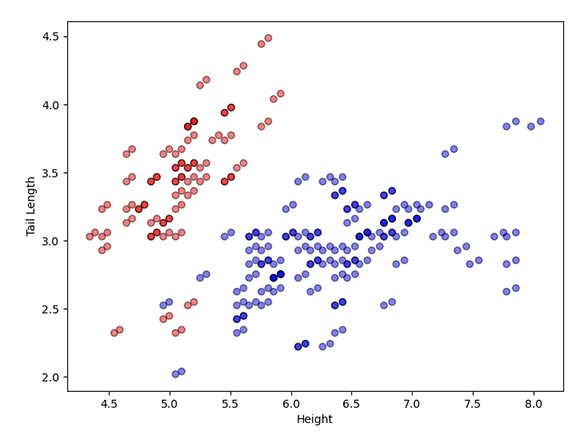
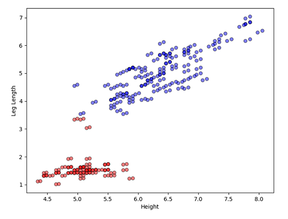
Figure 3.1. The results for the K-Means Clustering algorithm with two clusters, comparing height vs tail length (left) and height vs leg length (right).
Figure 3.1 depicts the comparisons between the two clusters. In the first image (left), we compare the height against the tail length. The results show that the algorithm has categorised the data into low height with medium to long-tail lengths (red) and medium to tall dogs with small to medium tail lengths (blue).
In the second image (right), we compare the height against the leg length. The first cluster (red) has detected a correlation between the smallest to medium height and small leg lengths, and the second cluster (blue) indicates that dogs with longer legs are more likely to be taller.
Notice how some of the data points look like they are incorrectly classified. However, this isn't the case. We trained the dataset on four features, and the graphs can only display two of them at once. Unfortunately, it's difficult to visualise data in higher dimensions and can make diagrams hard to read, so instead, we focus on a smaller portion of variables.
Three Clusters
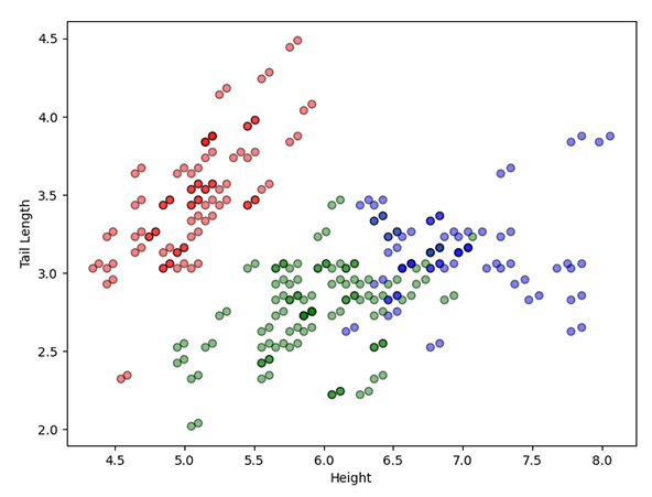
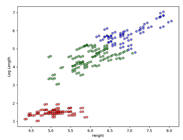
Figure 3.2. The results for the K-Means Clustering algorithm with three clusters, comparing height vs tail length (left) and height vs leg length (right).
In the three cluster examples (figure 3.2), we identify a better separation of dog breeds when compared to the two cluster examples. The first image (left) states medium-sized dogs are more likely to have longer tails (red). It continues with a second cluster (green), indicating that as the length of a dog's tail grows, so does its height. Interestingly, the blue clump contradicts the green one, identifying that large dogs will only have medium tail sizes.
In the second image (right), as the dog's height increases, so does the dog's leg length. The graph reveals a positive correlation between the two variables, best reflected through the three clusters: small (red), medium (green), and large (blue).
Error Trends
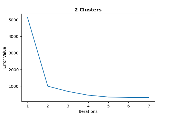
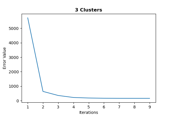
Figure 3.3. The graphs represent the error trend line for two and three clusters, respectively. They show the differences between the number of training iterations on the x-axis and the aggregated distance between each cluster on the y-axis.
Lastly, we discuss the error trend lines for the cluster variants (figure 3.3) to understand how the model performs during training. The two graphs are very similar, one for two clusters and the other for three, respectively. They compare the training iterations against the aggregated distance between each cluster during the iteration (objective function loss).
Notice how they show a decreasing trend in the error as the algorithm converges to optimality, indicating a robust model. Surprisingly, an additional cluster only increases the iteration count by two.
References
Dabbura, I. (2018) K-means Clustering: Algorithm, Applications, Evaluation Methods, and Drawbacks. Towards Data Science. Available from: https://towardsdatascience.com/k-means-clustering-algorithm-applications-evaluation-methods-and-drawbacks-aa03e644b48a